This tutorial introduces the scene graph data structure and Scene Window viewer.
Overview
The scene graph is a tree representing the local coordinate frames and objects in the scene. Each node in the scene graph represents a local coordinate frames. Edges in the scene graph indicate the relative transforms between local coordinate frames. Objects are represented in the scene graph as geometry, i.e., meshes or primitive shapes like boxes and spheres, attached to local coordinate frames. Both the environment and robot are represented in this same data structure. The frames for the environment will typically be fixed, while frames for robot joints will vary based on the robot's configuration.
Initial Example Scene
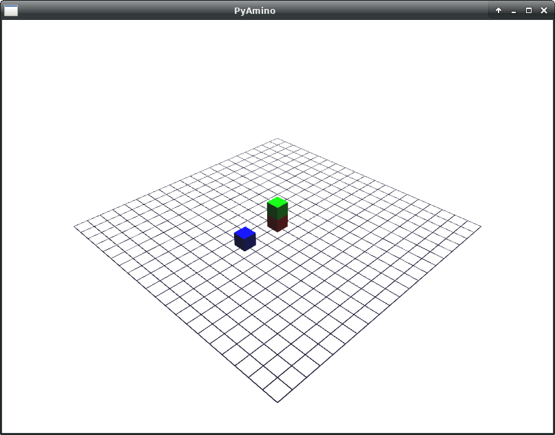
First, we will construct a simple scene containing a few boxes and a grid. The scene looks like the following:
Structurally, we will arrange the local coordinate frames as shown in the following:
There is a single root frame, labeled the code as empty string "". Child of the root is a frame for the grid. Red box A and blue box C are placed on the grid, so their frames are children of the grid. Green box B is placed on box A, so B is a child of A.
The following code constructs the scene and displays in the viewer:
#!/usr/bin/env python3
# File: t3-scene.py
# =================
#
# Create a scene with a grid and three boxes. Display the scene in
# the viewer window.
from amino import SceneWin, SceneGraph, Geom, QuatTrans
# Create a window
win = SceneWin(start=False)
# Create an (empty) scene graph
sg = SceneGraph()
# Draw a grid
sg.add_frame_fixed(
"",
"grid",
geom=Geom.grid({
"color": (0, 0, 1)
}, [1.0, 1.0], [.1, .1], .005))
# Draw some boxes
h = .1 # box height
dim = [h, h, h] # box dimension
sg.add_frame_fixed(
"grid",
"box-a",
tf=QuatTrans((1, (0, 0, h / 2))),
geom=Geom.box({
"color": (1, 0, 0)
}, dim))
sg.add_frame_fixed(
"box-a",
"box-b",
tf=QuatTrans((1, (0, 0, h))),
geom=Geom.box({
"color": (0, 1, 0)
}, dim))
sg.add_frame_fixed(
"grid",
"box-c",
tf=QuatTrans((1, (3 * h, 0, h / 2))),
geom=Geom.box({
"color": (0, 0, 1)
}, dim))
# Initalize the scene graph
sg.init()
# Pass the scenegraph to the window
win.scenegraph = sg
# Start the window in the current (main) thread
win.start(False)
Click and drag the mouse and to rotate the view, and zoom with the scroll wheel. Close the window the exit.
Robot Scene
Next, we will procedurally construct a serial robot. We model robots as chains or trees of local coordinate frames:
Each joint corresponds to a frame whose transform is parameterized by a configuration variable (i.e., the joint angle). In other words, the joint angle tells us the relative transform between a joint's local coordinate frame and the joint's parent frame. For each rigid body or link in the robot, we represent the points of that link in the link's local coordinate frame.
Robot Joints
The most common types of joints are revolute (rotating) and prismatic (linear).
Prismatic Joints
Prismatic joints create a linear motion. We compute the relative translation along the axis of motion:
\[ \setrans = \ell \unitvec{u} \; . \]
Revolute Joints
Revolute joints create a rotating motion. We compute the relative rotation about the axis of motion from the quaternion exponential
The following table summarizes the relative rotation and translation for these joints. The joint frame is labeled c and its parent p. For the revolute frame, we compute the rotation quaternion via the exponential; the translation \( \tf{\vec{v}}{p}{c} \) is constant. For the prismatic frame, rotation \(\tf{\quat{h}}{p}{c}\) is constant and we compute translation along the joint axis \(\vec{u}\).
Type
Rotation
Translation
Diagram
Revolute
\(\exp \left( \frac{\theta}{2}\vec{u} \right)\)
\( \tf{\vec{v}}{p}{c} \)
Prismatic
\(\tf{\quat{h}}{p}{c}\)
\( \ell \vec{u} \)
Example Robot Construction
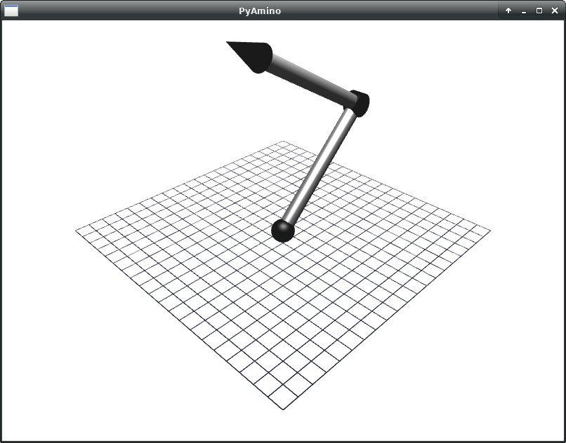
We will construct the following robot:
This robot has four joints: three at the shoulder and one at the elbow. For each joint, we create a "revolute" (rotating) frame and specify the joint's axis of rotation. To represent the robot's links, we attach geometry, i.e., a sphere, cylinders, and a cone, to various frames.
The following code constructs the robot, displays it in the viewer, and waves the elbow:
#!/usr/bin/env python3
# File: t3.1-robot.py
# ===================
#
# Procedural construction of a robot scene.
from math import pi, cos
from time import sleep
from amino import SceneWin, SceneGraph, Geom, GeomOpt, Vec3, YAngle, XAngle
def draw_robot(sg, parent):
"""Draw a robot in the scenegraph sg under parent"""
geom=Geom.cylinder(joint_opts, 2 * radius, r * radius))
sg.add_frame_fixed(
"e",
"lower-link",
tf=(YAngle(pi / 2), Vec3.identity()),
geom=Geom.cylinder(link_opts, len1, radius))
# "Hand"
sg.add_frame_fixed(
"e",
"hand",
tf=(YAngle(.5 * pi), (len1, 0, 0)),
geom=Geom.cone(joint_opts, 2 * (r**2) * radius, r * radius, 0))
sg.init()
# Create an (empty) scene graph
sg = SceneGraph()
# Draw a grid
sg.add_frame_fixed(
"",
"grid",
geom=Geom.grid({
"color": (0, 0, 1)
}, [1.0, 1.0], [.1, .1], .005))
# Draw the robot
draw_robot(sg, "grid")
# Initialize the scene graph
sg.init
# Create a window and pass the scenegraph
win = SceneWin(start=False)
win.scenegraph = sg
# Start the window in a background thread
win.start(True)
# Do a simple wave
dt = 1.0 / 60
t = 0
while win.is_runnining():
t += dt
e_angle = (120 + 15 * cos(t)) * (pi / 180)
win.config = {"s1": -.75 * pi, "e": e_angle}
sleep(dt)
Scene Compiler
Finally, we will use the scene compiler to generate a plugin (shared library) for a scene. The scene compilers supports definitions in a block-oriented (curly-braced) syntax and in URDF.
Scene Files
We will redefine our serial robot in a scene file, compile the scene, and load it in the viewer.
Use the following scene file:
/* example.roboray
* ===============
*
* Serial robot example in a scene file.
*/
/* Parameters for the robot */
def rad 0.05; // Link radius
def len0 1; // upper arm length
def len1 1; // forearm length
def r 1.618; // a ratio
/* Define classes for robot parts */
class link {
shape cylinder;
radius rad;
color [.5, .5, .5];
specular [2, 2, 2];
}
class joint_style {
color [0, 0, 0];
specular [.5, .5, .5];
}
/* Draw the grid */
frame grid {
geometry {
shape grid;
delta [.1, .1];
thickness .005;
dimension [1, 1];
}
}
/* Draw the robot */
// Shoulder
frame s0 {
type revolute; # frame type: revolute joint
axis [1, 0, 0]; # joint axis
geometry {
isa joint_style; # instance of joint_style class
shape sphere;
radius r*rad;
}
}
frame s1 {
parent s0;
type revolute;
axis [0, 1, 0];
}
frame s2 {
parent s1;
type revolute;
axis [1, 0, 0];
// nested frame is a child of s2
frame upper-link {
rpy [0, pi/2, 0];
geometry {
isa link;
height len0;
}
}
}
// Elbow
frame e {
parent s2;
type revolute;
axis [0,1,0];
translation [len0, 0, 0];
frame e-link {
rpy [pi/2, 0, 0];
translation [0, rad, 0];
geometry {
isa joint_style;
shape cylinder;
height 2*rad;
radius r*rad;
}
}
frame lower-link {
rpy [0, pi/2, 0];
geometry {
isa link;
height len1;
}
}
// "Hand"
frame hand {
rpy [0, pi/2, 0];
translation [len1, 0, 0];
geometry {
shape cone;
height 2*r*r*rad;
start_radius r*rad;
end_radius 0;
}
}
}
Use the scene compiler to build the plugin. While you may call the scene compiler directly from the shell, it will be preferable to use a build script. The following CMake file will build a plugin for the serial robot:
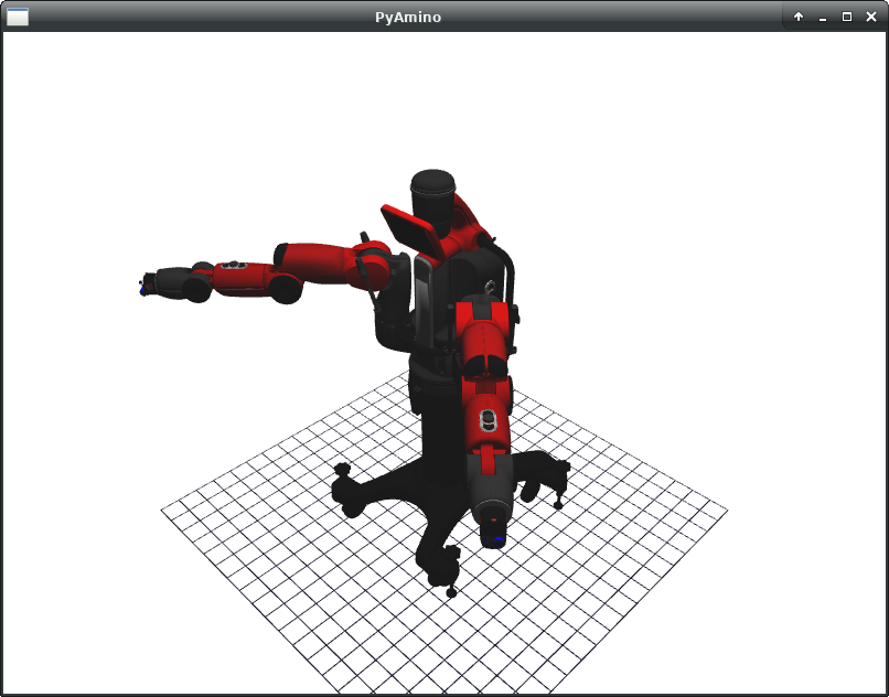
Now, check that you can load the Baxter model. The following command will visualize the Baxter in the viewer. Click and drag the mouse and to rotate the view, and zoom with the scroll wheel. Close the window the exit.
From the directory containing the CMakLists.txt, build the plugin by running:
cmake .
make
The command will generate a C file baxter-model.c from the URDF. Then, it will compile the baxter model into the plugin libbaxter-model.so which describes the kinematic layout and all meshes of the robot.